NOTE: This guide is currently a work in progress.
Introduction
Kalman filters let you use mathematical models despite having error-filled real-time measurements. Programmers dealing with real-world data should know them. Publications explaining Kalman filters are hard for Computer Scientists/Engineers to understand since they expect you to know control theory. I wrote this guide for people who want to learn Kalman filters but never took a control theory course.
DISCLAIMER: This guide teaches amateur-level Kalman filtering for hobbyists. If lives depend on your Kalman filter (such as manned aviation, ICBMs, medical instruments, etc), do not rely on this guide! I skip a lot of details necessary for serious use!
This guide will cover:
- When Kalman filters can help.
- Examples of solving simple problems with Kalman filters.
- Examples of how to convert normal-looking equations into Kalman filter matrices.
- Example code implementing Kalman filters in Python.
This guide WON'T cover:
- Kalman filter history. Please consult the University of North Carolina at Chapel Hill's great website for information on this subject.
- When and why Kalman filters are optimal.
- How to tune Kalman filters for performance.
- In-depth details (such as exceptions to guidelines).
This guide aims to quickly get you 80% of the way toward understanding Kalman filters. I won't cover the remaining 20% since that's not the point of this guide. If you need to know Kalman filters to that depth, find a more detailed guide.
When Can Kalman Filters Help?
Kalman filters can help when four conditions are true:
- You can get measurements of a situation at a constant rate.
- The measurements have error that follows a bell curve.
- You know the mathematics behind the situation.
- You want an estimate of what's really happening.
There are exceptions, but I'll let other publications explain them.
Linear Kalman Filters
Prerequisites
To understand these linear Kalman filter examples, you will need a basic understanding of:
- High school physics
- Matrix algebra
- Python for the programming parts.
Basics
Here are the most important concepts you need to know:
- Kalman Filters are discrete. That is, they rely on measurement samples taken between repeated but constant periods of time. Although you can approximate it fairly well, you don't know what happens between the samples.
- Kalman Filters are recursive. This means its prediction of the future relies on the state of the present (position, velocity, acceleration, etc) as well as a guess about what any controllable parts tried to do to affect the situation (such as a rudder or steering differential).
- Kalman Filters work by making a prediction of the future, getting a measurement from reality, comparing the two, moderating this difference, and adjusting its estimate with this moderated value.
- The more you understand the mathematical model of your situation, the more accurate the Kalman filter's results will be.
- If your model is completely consistent with what's actually happening, the Kalman filter's estimate will eventually converge with what's actually happening.
When you start up a Kalman Filter, these are the things it expects:
- The mathematical model of the system, represented by matrices A, B, and H.
- An initial estimate about the complete state of the system, given as a vector x.
- An initial estimate about the error of the system, given as a matrix P.
- Estimates about the general process and measurement error of the system, represented by matrices Q and R.
During each time step, you are expected to give it the following information:
- A vector containing the most current control state (vector "u"). This is the system's guess as to what it did to affect the situation (such as steering commands).
- A vector containing the most current measurements that can be used to calculate the state (vector "z").
After the calculations, you get the following information:
- The most current estimate of the true state of the system.
- The most current estimate of the overall error of the system.
The Equations
NOTE: The equations are here for exposition and reference. You aren't expected to understand the equations on the first read.
The Kalman Filter is like a function in a programming language: it's a process of sequential equations with inputs, constants, and outputs. Here I've color-coded the filter equations to illustrate which parts are which. If you are using the Kalman Filter like a black box, you can ignore the gray intermediary variables.
BLUE = inputs ORANGE = outputs BLACK = constants GRAY = intermediary variables
|
State Prediction (Predict where we're gonna be) |
 |
|
Covariance Prediction (Predict how much error) |
 |
|
Innovation (Compare reality against prediction) |
 |
|
Innovation Covariance (Compare real error against prediction) |
 |
|
Kalman Gain (Moderate the prediction) |
 |
|
State Update (New estimate of where we are) |
 |
|
Covariance Update (New estimate of error) |
 |
Inputs:
Un = Control vector. This indicates the magnitude of any control system's or user's control on the situation.
Zn = Measurement vector. This contains the real-world measurement we received in this time step.
Outputs:
Xn = Newest estimate of the current "true" state.
Pn = Newest estimate of the average error for each part of the state.
Constants:
A = State transition matrix. Basically, multiply state by this and add control factors, and you get a prediction of the state for the next time step.
B = Control matrix. This is used to define linear equations for any control factors.
H = Observation matrix. Multiply a state vector by H to translate it to a measurement vector.
Q = Estimated process error covariance. Finding precise values for Q and R are beyond the scope of this guide.
R = Estimated measurement error covariance. Finding precise values for Q and R are beyond the scope of this guide.
To program a Kalman Filter class, your constructor should have all the constant matrices, as well as an initial estimate of the state (x) and error (P). The step function should have the inputs (measurement and control vectors). In my version, you access outputs through "getter" functions.
Here is a working Kalman Filter object, written in Python:
Single-Variable Example
Situation
This is a classic example. We will attempt to measure a constant DC voltage with a noisy voltmeter. We will use the Kalman filter to filter out the noise and converge toward the true value.
The state transition equation:

Vn = The current voltage.
Vn-1 = The voltage last time.
Wn = Random noise (measurement error).
Since the voltage never changes, it is a very simple equation. The objective of the Kalman filter is to mitigate the influence of Wn in this equation.
Simulation
In Python, we simulate this situation with the following object:
Preparation
The next step is to prepare the Kalman filter inputs and constants. Since this is a single-variable example, all matrices are 1x1.
Matrix "A" is what you need to multiply to last time's state to get the newest state. Since this is a constant voltage, we just multiply by 1.

A = 1
Matrix "H" is what you need to multiply the incoming measurement to convert it to a state. Since we get the voltage directly, we just multiply by 1.
H = 1
Matrix "B" is the control matrix. It's a constant voltage and there's no input in the model we can change to affect anything, so we'll set it to 0.
B = 0
Matrix "Q" is the process covariance. Since we know the exact situation, we'll use a very small covariance.
Q = 0.00001
Matrix "R" is the measurement covariance. We'll use a conservative estimate of 0.1.
R = 0.1
Matrix "xhat" is your initial prediction of the voltage. We'll set it to 3 to show how resilient the filter is.
xhat = 3
Matrix "P" is your initial prediction of the covariance. We'll just pick an arbitrary value (1) because we don't know any better.
P = 1
Execution and Python code

For brevity, I don't list all the code in this guide. The complete file is available: kalman1.py . I highly recommend you read through it and play with the starting values.
NOTE: The single-variable example is for simple illustrative purposes only. For a real-world project involving smoothing out a single variable of time-series data, I would suggest using a low-pass filter. It's a lot less coding for basically the same result. If you absolutely need a one-dimensional Kalman filter for smoothing signals out, there is an excellent tutorial with simpler notation and C code.
Multi-Variable Example
Situation
We will use a common physics problem with a twist. This example will involve firing a ball from a cannon at at 45-degree angle at a muzzle velocity of 100 units/sec. However, we will also have a camera that will record the ball's position from the side every second. The positions measured from the camera have significant measurement error. We also have precise detectors in the ball that give the X and Y velocity every second.
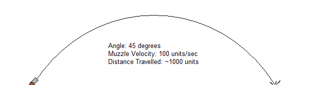
(not drawn to scale)
The kinematic equations for this situation, done to death in physics classes around the world, are:

Our filter is discrete. Let's convert these equations to a recurrence relation, with delta-t being a fixed time step:

These equations can be represented in an alternate form shown here:

Note that rows are the summation of the influence of the variables in each column. This notation will be important to illustrate something in the Preparation step, so remember it.
Simulation
We will simulate the cannonball's trajectory mid-flight with the following Python object:
Preparation
Remember this alternate form of the kinematic equations I showed you?
The first part is A in disguise (with the variables removed), and the second part is the control vector, provided you use the B matrix shown here:
Compare:
to:

When a state is multiplied by H, it is converted to measurement notation. Since our measurements map directly to the state, we just have to multiply them all by 1 to convert our measurements to state:

X0 is the initial guess for the ball's state. Notice that this is where we break the muzzle velocity into its X/Y components. We're also going to set y way off on purpose to illustrate how fast the filter can deal with this:

P is our initial guess for the covariance of our state. We're just going to set them all to 1 since we don't know any better (and it works anyway). If you want to know better, consult a more detailed guide.
Q is our estimate of the process error. Since we created the process (the simulation) and mapped our equations directly from it, we can safely assume there is no process error:

R is our estimate of the measurement error covariance. We'll just set them all arbitrarily to 0.2. Try playing with this value in the real code.

Execution and Python code

That's a pretty good estimate, given how much error our measurements have!
The complete code for this example is available at: kalman2.py
Conclusion
I hope that this guide was useful to you. This is a living document. If you have any suggestions, comments, etc, please send me a message at greg {at] czerniak (dot} info so I can make this guide even better. ESPECIALLY send me a message if you got confused somewhere -- you're probably not the first or last person that will get hung up at that point.
References
Kalman Filters
- The Kalman Filter: A great launching point for information about the Kalman filter.
- Kalman Filter: Wikipedia page. I modified the equations from this page for my version.
- Simultaneous Localization and Mapping (SLAM) : Seeing the matrices in the PowerPoint slides inspired me to write this guide. Most of my examples are variations of examples in these slides.
- A 3D State Space Formulation of a Navigation Kalman Filter for Autonomous Vehicles : This text goes in-depth about using Kalman filters in robotics, and it has great introductory material.
- Optimal Filtering : This book goes into detail on using Kalman filters.
Tools
- Latex2png, latex2gif, latex2eps, latex2jpg : This site generates image files from LaTeX code.
- PBworks : This is how I organize my thoughts.
Special Thanks
- Special thanks to Stefan Wollny from Korea for detecting and reporting a variance/covariance typo.
- Special thanks to Dave Bloss of Topsfield, Massachusetts and Robby Nevels for detecting and reporting a mistake with the cannonball physics equations (1/2gt^2 instead of gt^2).
- Special thanks to Robby Nevels for detecting and reporting a mistake with the Kalman filter code (innovation was being calculated wrong).